14 - Simple Linear Regression

14.1 Simple Linear Regression Model

Regression Model and Regression Equation

Regression analysis requires us to develop a regression model, an equation showing how a dependent variable \( y \) is related to the independent variable \( x \).

The simple linear regression model is as follows:

\[ y = \beta _0 + \beta _1 x + \epsilon \]

Where \( \beta _0 \) and \( \beta _1 \) are referred to as the parameters of the model, and \( \epsilon \) is a random variable called the error term. The error term accounts for the variability in y cannot be explained by the linear relationship between \( x \) and \( y \).

The equation that describes how the expected value of \( y \), denoted \( E(y) \), is related to \( x \) is called the regression equation:

\[ E(y) = \beta _0 + \beta _1 x \]

Note that this model is a line with slope \( \beta _1 \) and y-intercept \( \beta _0 \).

Estimated Regression Equation

Since the values of the population parameters \( \beta _0 \) and \( \beta _1 \) are rarely known, they must be estimated. These estimates are represented as the sample statistics \( b_0 \) and \( b_1 \). With this, we can now construct the estimated regression equation:

\[ \hat{y} = b_0 + b_1 x \]

The graph of this equation is known as the estimated regression line.

14.2 Least Squares Method

The least squares method is a procedure for using sample data to find the estimated regression equation. This method uses sample data to provide the values of \(b_0\) and \(b_1\) that minimize the sum of the squares of the deviations between the observed values of the dependent variable \(y_i\) and the predicted values of the dependent variable \(\hat{y}_i\):

\[ min\ \Sigma (y_i - \hat{y}_i)^2 \]

where

• \(y_i\) = observed value of the dependent variable for the ith observation

• \(\hat{y}_i\) = predicted value of the dependent variable for the ith observation.

Using calculus, you can derive the following equations for \(b_0\) and \(b_1\):

\[ b_1 = \frac{\Sigma (x_i - \bar{x})(y_i - \bar{y})}{\Sigma (x_i - \bar{x})^2} \]

\[ b_0 = \bar{y} - b_1 \bar{x} \]

where

• \(x_i\) = value of the independent variable for the ith observation

• \(y_i\) = value of the dependent variable for the ith observation

• \(\bar{x}\) = mean value for the independent variable

• \(\bar{y}\) = mean value for the dependent variable

• \(n\) = total number of observations

14.3 Coefficient of Determination

The coefficient of determination provides a measure of the goodness of the fit for an estimated regression equation.

For the ith observation, the difference between the observed value of the dependent variable (\(y_i\)) and the predicted value of the dependent variable (\(\hat{y}_i\)) is called ith residual (\(y_i - \hat{y}_i\)). The ith residual represents the error in using \(\hat{y}_i\) to estimate \(y_i\). The sum of squares of these residuals or errors is the quantity that is minimized in the least squares method. This quantity is known as the sum of squares due to error (SSE).

\[ SSE = \Sigma (y_i - \hat{y}_i)^2 \]

The value of SSE is a measure of the errror in using the estimated regression equation to predict the value of the dependent variable in a sample.

When we don’t know the size of the population, we must also estimate the population mean with the sample mean. The error due to this can be calculated as the total sum of squares (SST).

\[ SST = \Sigma (y_i - \bar{y})^2 \]

Note that we can think of SSE as a measure of how well the observations cluster above the line \( y=\hat{y} \) and SST as a measure of how well the observations cluster above the line \( y=\bar{y} \).

The sum of squares due to regression (SSR) is a measure of how much the values of \(\hat{y}\) deviate from \(\bar{y}\):

\[ SSR = \Sigma (\hat{y}_i - \bar{y})^2 \]

Theses 3 values are related as such:

\[ SST = SSR + SSE \]

The coefficient of determination (\(r^2\)) measures the goodness of fit for the estimated regression equation. Note that \(r^2\) will always have a value between 0 and 1.

\[ r^2 = \frac{SSR}{SST} = 1 - \frac{SSE}{SST} \]

Correlation Coefficient

The correlation coefficient (\(r_{xy}\)) is a descriptive measure of the strength of linear association between two variables \(x\) and \(y\). Note that the values of \(r_{xy}\) lie between -1 and 1 where negative values of \(r_{xy}\) indicate a negative relationship between \(x\) and \(y\) and positive and positive values of \(r_{xy}\) indicate a positive relationship between \(x\) and \(y\).

\[ r_{xy} = (sign\ of\ b_1)\sqrt{r^2} \]

14.4 Model Assumptions

The tests of significance in regression analysis are based off on the following assumptions of the error term \(\epsilon\):

1. \(E(\epsilon) = 0\). This is necessary so that the expected value of the simple linear regression model \(y = \beta _0 + \beta _1 x + \epsilon\) works itself out to be \(y = \beta _0 + \beta _1 x\).

2. The variance of \(\epsilon\), denoted by \(\sigma^2\), is the same for all values of \(x\).

3. The values of \(\epsilon\) are independent.

4. The error term \(\epsilon\) is a normally distributed random variable for all values of \(x\).

Note that linear regression also assumes that relationships between the variables analyzed is in fact linear.

14.5 Testing for Signifance

In a linear regression equation, we can demonstrate that there is no linear relationship if \(\beta_1 = 0\). To test the significance of the linear relationship, we must conduct a hypothesis test to determine if \(\beta_1 = 0\). These tests require an estimate of \(\sigma^2\), which is the variance of \(\epsilon\).

Estimate of \(\sigma^2\)

From the assumptions of the regression model, we can assume that \(\sigma^2\) represents the variance of the \(y\) values about the regression line. This means that the SSE is a measure of the variability of the actual observations about the estimated regression line. The mean square error (MSE) provides the estimate of \(\sigma^2\), which is the SSE divided by its degrees of freedom. SSE has \(n-2\) degrees of freedom since two parameters (\(\beta_0\) and \(\beta_1\)) must be estimated.

\[ s^2 = MSE = \frac{SSE}{n-2} \]

We can then find the standard error of the estimate (\(s\)).

\[ s = \sqrt{MSE} = \sqrt{\frac{SSE}{n-2}} \]

\(t\) Test

To test if \(x\) and \(y\) are linearly related, we must conduct a hypothesis test:

\[ H_0 : \beta_1 = 0 \]

\[ H_a : \beta_0 \neq 0 \]

We must remember that the estimators of the linear regression equation are sampling statistics with their own sampling distributions.

\[ E(b_1) = \beta_1 \]

\[ \sigma _{b_1} = \frac{\sigma}{\sqrt{\Sigma (x_i - \bar{x})^2}} \]

However, we must estimate the value of \(\sigma _{b_1}\) since we do not know the value of \(\sigma\):

\[ s_{b_1} = \frac{s}{\sqrt{\Sigma (x_i - \bar{x})^2}} \]

The \(t\) test for significance in the relationship is based on the following test statistic with \(n-2\) degrees of freedom:

\[ \frac{b_1 - \beta_1}{s_{b_1}} \]

If the null hypothesis is true, then \(\beta_1 = 0\) and the test statistic will be:

\[ \frac{b_1}{s_{b_1}} \]

Confidence Interval for \(\beta_1\)

The confidence interval for \(\beta_1\) with confidence level \(1-\alpha\) is given as follows:

\[ b_1 \pm t_{\alpha/2}s_{b_1} \]

Note that the \(t\) distribution has \(n-2\) degrees of freedom.

\(F\) Test

With only one independent variable, an \(F\) test will provide the same conclusion as \(t\) test. However, an \(F\) test can test for an overall significant relationship in cases with more than one independent variables.

The mean squares due to regression (MSR) provides another estimate of \(\sigma^2\).

\[ MSR = \frac{SSR}{Regression\ degrees\ of\ freedom} \]

For the models covered in our situtations, the regression degrees of freedom are always equal to the number of independent variables in the model.

The test statistic in an \(F\) test is as follows:

\[ F = \frac{MSR}{MSE} \]

If \(H_0:\beta_1=0\) is true, then MSR and MSE are independent estimators of \(\sigma^2\) and the sampling distribution of MSR/MSE follows an \(F\) distribution with numerator degrees of freedom equal to 1 and denominator degrees of freedom equal to \(n-2\). Therefore, when the null hypothesis is true, the value of MSR/MSE should be close to 1. Alternatively, large values of MSR/MSE will lead to a rejection of the null hypothesis.

14.6 Using the Estimated Regression Equation for Estimation and Prediction

When using the estimated regression equation to estimate the mean value of \(y\) or predict an individual value of \(y\), we use the following notation:

• \(x^*\) = the given value of the independent variable \(x\)

• \(y^*\) = the random variable denoting the possible values of the dependent variable \(y\) when \(x=x^*\)

• \(E(y^*)\) = the mean or expected value of the dependent variable \(y\) when \(x=x^*\)

• \(\hat{y}^*\) = \(b_0+b_1x^*\) = the point estimator of \(E(y^*)\) and the predictor of an individual value of \(y^*\) when \(x=x^*\)

Interval Estimation

A confidence interval is an interval estimate of the mean value of \(y\) for a given value of \(x\).

A prediction interval is used whenever we want to predict an individual value of \(y\) for a new observation corresponding to a given value of \(x\). Note that the margin of error is larger for a prediction interval than a confidence interval.

Confidence Interval for the Mean Value of \(y\)

If we want to make an inference about how close \(\hat{y}^*\) is to the true mean value \(E(y^*)\), we have to estimate the variance of \(\hat{y}^*\):

\[ s_{\hat{y}^*}^2 = s^2\left[\frac{1}{n} + \frac{(x^*-\bar{x})^2}{\Sigma(x_i-\bar{x})^2}\right] \]

To estimate the standard deviation of \(\hat{y}^*\):

\[ s_{\hat{y}^*} = s\sqrt{\frac{1}{n} + \frac{(x^*-\bar{x})^2}{\Sigma(x_i-\bar{x})^2}} \]

The margin of error associated with this confidence interval is \(t_{\alpha/2}s_{\hat{y}^*}\), so it follows that confidence interval for \(E(y^*)\) is:

\[ \hat{y}^* \pm t_{\alpha/2}s_{\hat{y}^*} \]

where the confidence coefficient is \(1-\alpha\) and \(t_{\alpha/2}\) is based on the \(t\) distribution with \(n-2\) degrees of freedom.

Prediction Interval for an Individual Value of \(y\)

To develop a prediction interval, we must first determine the variance associated with using \(\hat{y}^*\) as a predictor of \(y\) when \(x=x^*\). This variance is the sum of 2 components:

1. The variance of \(y^*\) values about the mean \(E(y^*)\), an estimate which is given by \(s^2\)

2. The variance associated with using \(\hat{y}^*\) to estimate \(E(y^*)\), an estimate which is given by \(s_{\hat{y}^*}^2\)

The formula for estimating the variance corresponding to the prediction of the value of \(y\) when \(x=x^*\), denoted \(s_{pred}^2\), is:

\[\begin{split} \begin{align} s_{pred}^2 &= s^2 + s_{\hat{y}^*}^2 \\ &= s^2 + s^2 \left[ \frac{1}{n} + \frac{(x^2-\bar{x})^2}{\Sigma(x_i-\bar{x})^2} \right] \\ &= s^2 \left[ 1 + \frac{1}{n} + \frac{(x^*-\bar{x})^2}{\Sigma(x_i-\bar{x})^2} \right] \end{align} \end{split}\]

It follows that the standard deviation corresponding to the prediction of the value of \(y^*\) is:

\[ s_{pred} = s \sqrt{1 + \frac{1}{n} + \frac{(x^*-\bar{x})^2}{\Sigma(x_i-\bar{x})^2}} \]

Since the margin of error associated with the prediction interval is \(t_{\alpha/2}s_{pred}\), the prediction interval for \(y^*\) is:

\[ \hat{y}^* \pm t_{\alpha/2}s_{pred} \]

where the confidence coefficient is \(1-\alpha\) and \(t_{\alpha/2}\) is based on a \(t\) distribution with \(n-2\) degrees of freedom.

14.7 Excel’s Regression Tool

The following steps describe how to use Excel’s regression tools:

1. Click the Data tab on the Ribbon

2. In the Analyze group, click Data Analysis

3. Choose Regression from the list of Analysis Tools

4. When the Regression dialog box appears:

   • Enter values in the Input Y Range: and Input X Range: boxes

   • Select the check box for Labels

   • Select the check box for Confidence Level: and enter the confidence level

   • Select Output Range: in the Output options area and enter top-left cell of the section where you want the output to appear

   • Click OK

14.8 Residual Analysis: Validating Model Assumptions

Residual analysis is the primary tool for determining if whether the assumed regression model is appropriate. Remember that a residual is just the difference between the observed and expected value (\(y_i-\hat{y}_i\)).

Recall the equation upon which the simple linear regression model is based (\(y = \beta_0 + \beta_1 x + \epsilon\)). Residual analysis allows us to measure the error term \(\epsilon\).

Much of residual analysis is based on an examination of graphical plots:

1. A plot of the residuals against values of the independent variable \(x\)

2. A plot of residuals against the predicted values of the dependent variable \(y\)

3. A standardized residual plot

4. A normal probability plot

Residual Plot Against \(x\)

A residual plot against the independent variable \(x\) is a graph in which the values of the independent variable are represented by the the horizontal axis and the corresponding residual values are represented by the vertical axis. A point is plotted for each residual \((x_i,y_i-\hat{y}_i)\).

The resulting graph might indicate that the fit is good if the residuals cluster around the \(x\)-axis. If the residuals instead form a triangle or similar shape around the \(x\)-axis, this might indicate non-constant variance. If another shape, such as a parabola appears, this might indicate that the model form is inadequate.

Residual Plot Against \(\hat{y}\)

This plot estimated value of the independent variable \(\hat{y}\) as the \(x\)-axis and the value of the residual \(y_i-\hat{y}_i\) as the \(y\)-axis.

Note that the same insights can be drawn from the shape of this graph as that of the residual plot against \(x\). However, this version is more useful in multiple regression analysis.

Standardized Residuals

A random variable can be standardized by subtracting its mean and dividing by its standard deviation. Since the least squares method quarantees that the mean of the residuals is 0, we can find the standardized residual by dividing the residual by its standard deviation.

To find the standard deviation of the ith residual:

\[ s_{y_i-\hat{y}_i} = s \sqrt{1-h_i} \]

where

• \(s_{y_i-\hat{y}_i}\) = the standard deviation of residual i

• \(s\) = the standard error of the estimate

• \(h_i\) = \(\frac{1}{n} + \frac{(x_i-\bar{x})^2}{\Sigma(x_j-\bar{x})^2}\)

Once we’ve calculated the standard deviation of the ith residual, we can compute the standardized residual:

\[ \frac{y_i-\hat{y}_i}{s_{y_i-\hat{y}_i}} \]

The standardized residual plot can provide insight about the assumption that the error term \(\epsilon\) has a normal distribution. If this assumption is satisfied, then the distribution should appear to come from a standard normal probability distribution (i.e. with a 95% confidence interval, most values should fall between \(-2\) and \(2\)).

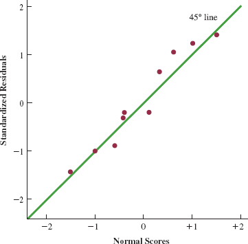
Normal Probability Plot

Another approach to determining the validity of the assumption that the error term has a normal distribution is the normal probability plot. To show how this concept is developed, we must use normal scores.

Normal scores are order statistics that represent the expected value that for each ordered item when sampling from a standard normal distribution:

For example, with \(n=10\):

Order Statistic	Normal Score
1	-1.55
2	-1.00
3	-0.65
4	-0.37
5	-0.12
6	0.12
7	0.37
8	0.65
9	1.00
10	1.55

We can then compare the normal scores to the ordered standard residuals to see if the distribution of \(\epsilon\) is approximately normal:

Order Statistic	Normal Score	Ordered Standard Residuals
1	-1.55	-1.7114
2	-1.00	-1.0792
3	-0.65	-0.9487
4	-0.37	-0.2372
5	-0.12	-0.2296
6	0.12	-0.2296
7	0.37	0.7115
8	0.65	1.0792
9	1.00	1.2224
10	1.55	1.4230

14.9 Outliers and Influential Observations

Detecting Outliers

An outlier is a data point that does not fit the trend shown by the remaining data. They often indicate either erroneous data or incorrect model assumptions.

The standardized residuals are often the best method of detecting outliers. Take note of any standardized residuals outside of the range \([-2,2]\).

Additionally, plotting the points often makes outliers apparent.

Detecting Influential Observations

An influential observation is an observation that has a strong influence on the regression results. These may be due to outliers or extreme \(x\) values.

Observations with extreme values for the independent variables are called high leverage points. The leverage of an observation is given by:

\[ h_i = \frac{1}{n} + \frac{(x_i-\bar{x})^2}{\Sigma(x_j-\bar{x})^2} \]